What is Microsoft Excel ? and Basic Workouts

 What is Microsoft Excel and About Excel.

What is Microsoft Excel?

Microsoft Excel is an office use application designed by Microsoft. It comes with Office Suite with several other Microsoft applications, such as Word, Powerpoint, Access, Outlook, and OneNote, etc. It is supported in Windows as well as Mac operating system too.

Microsoft Excel is one of the most suitable spreadsheet programs that help us to store and represent the data in tabular form, manage and manipulate data, create optically logical charts, and more. Excel provides you the worksheet to create a new document in it. You can save the Excel file with .xls extension.

Note: We are using Excel 2016 for this Excel tutorial.

Worksheet

A worksheet is made of rows and columns that intersect each other to form cells where data is entered. It is capable of performing multiple tasks like calculations, data analysis, and integrating data.

In Excel worksheet, rows are represented by numbers and columns by alphabets.

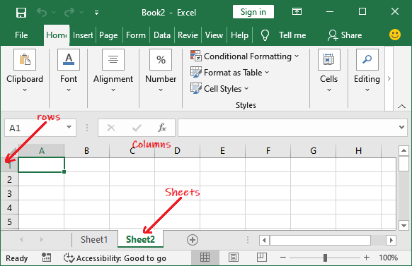
A single Excel workbook can consist of several sheets, named Sheet1, Sheet2, Sheet3… SheetN. You can add one or more sheets to your Excel document.

Microsoft Excel Features

There are several features that are available in Excel to make our task more manageable. Some of the main features are:

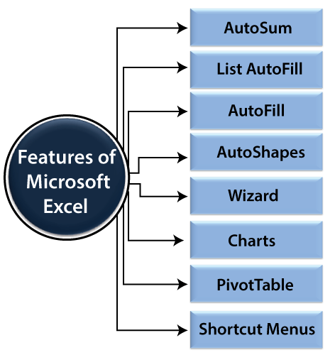
1. AutoFormat: It allows the Excel users to use predefined table formatting options.
2. AutoSum: AutoSum feature helps us to calculate the sum of a row or column automatically by inserting an addition formula for a range of cells.
3. List AutoFill: It automatically develops cell formatting when a new component is added to the end of a list.
4. AutoFill: This feature allows us to quickly fill cells with a repetitive or sequential record such as chronological dates or numbers and repeated documents. AutoFill can also be used to copy functions. We can also alter text and numbers with this feature.
5. AutoShapes: AutoShapes toolbar will allow us to draw some geometrical shapes, arrows, flowchart items, stars, and more. With these shapes, we can draw our graphs.
6. Wizard: It guides us to work effectively while we work by displaying several helpful tips and techniques based on what we are doing. Drag and Drop feature will help us to reposition the record and text by simply dragging the data with the help of the mouse.
7. Charts: This feature will help you to present the data in graphical form by using Pie, Bar, Line charts, and more.
8. PivotTable: It flips and sums data in seconds and allows us to execute data analysis and generating documents like periodic financial statements, statistical documents, etc. We can also analyze complex data relationships graphically.
9. Shortcut Menus: The shortcut menu helps users to make the work done through shortcut commands that need a lengthy process.

How to Open Microsoft Excel?

In Windows 10 operating system, click on the Start button and search for the MS Excel application. If it is already installed in your system, it will appear here like this.

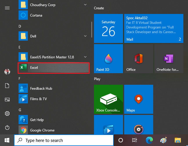
Double-tap on this icon to open the Excel.

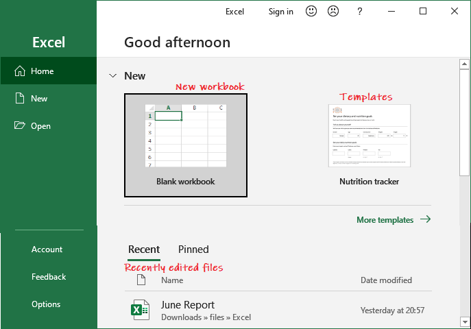
When the Excel opens, an interface will appear like this. From here, you can create a new workbook, choose a template, and access your recently edited workbooks.

Create a new workbook

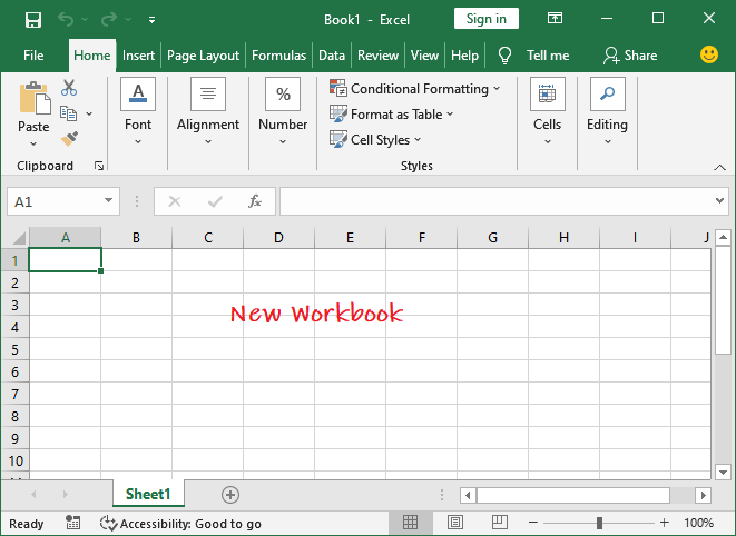
To create a new workbook, click on the Blank Workbook here.

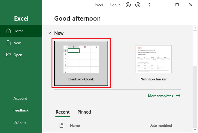
A blank Excel worksheet will open and display to you.

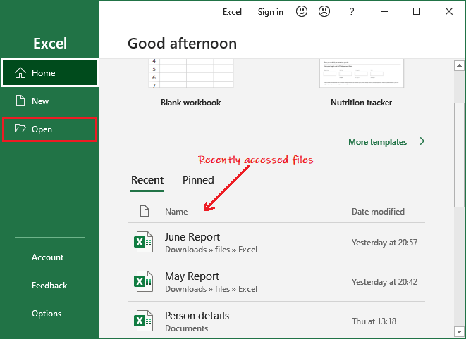
Open an existing workbook

If you want to work with an existing workbook, you can either choose from the Recent list or click on the Open button to select from the specific location.

When you click the Open button, it will ask you to open the existing file from different locations, such as - Recent, OneDrive, This PC, and Browse.

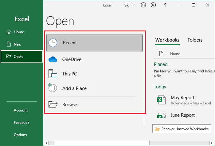
We will go for Browse this time; it will directly take you to the local computer location. From here, you can choose the Excel file you want to open.

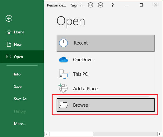
Choose a file from your computer and click on the Open button.

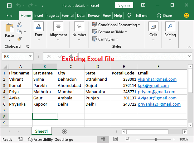
An existing Excel file that is stored on your local computer will open like this.

Setup the option to open the blank workbook automatically

In MS Excel, you can setup the option to open the blank Excel workbook by default whenever you start the Excel.

1. Click File then Options (Inside the More… in the right panel).
2. On the General tab, scroll down and go to the Start up options.
3. Here, uncheck the Shows the Start screen when this program starts checkbox and then click OK.
   
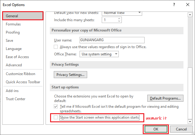
4. The next time you start Excel, it will open a blank workbook automatically.

Excel Interface

It is the main interface of an Excel worksheet, where we work and store our data. This interface contains various components. Before start working with Excel worksheet, you should be familiar with these components so that you can use the Excel application efficiently.

Once you get familiar with the Excel interface, you will able to identify the basic and most-used components of an Excel workbook. We have explained a bit about these components.

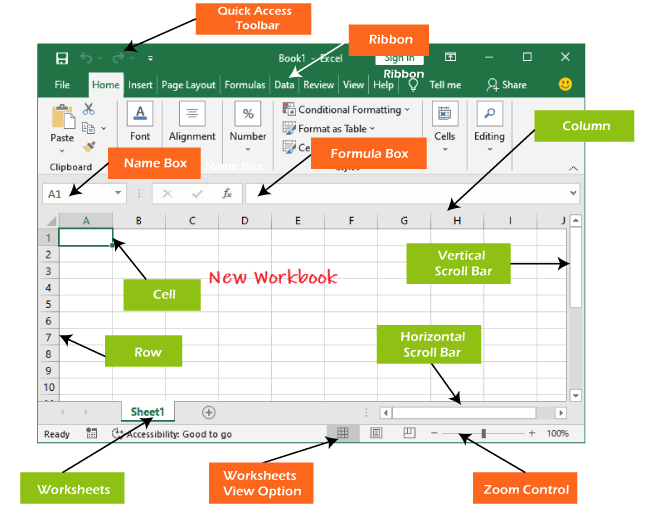
Quick Access Toolbar

The Quick Access Toolbar contains some common and most used commands of Excel, which users repeatedly need while working with Excel. By default, Save, Undo, and Repeat commands are added in the quick access toolbar.

It provides fast access to its users by adding most-used commands in it. This quick access toolbar is customizable. It means you can add other commands, whichever you need most.

Add commands to the Quick Access toolbar

Step 1: Click on the drop-down arrow to the right of the Quick Access toolbar.

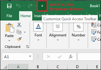
Step 2: Select the command you wish to add in the quick access toolbar from the drop-down menu.

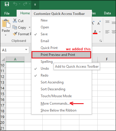
For more command, which is not available here, click on More Commands and choose from there.

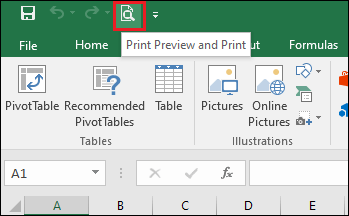
Step 3: Here, we have selected command Print Preview and Print that has been added to the Quick Access toolbar along with other commands. You can see it here.

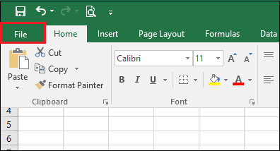
Excel Ribbon

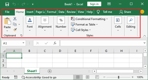
Excel 2016 utilizes a tabbed Ribbon system instead of traditional menus. The Ribbon includes multiple tabs, each with several groups of commands. We will use these tabs to perform the most common function in Excel.

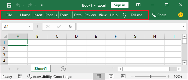
File, Home, Insert, Page Layout, Formula, Data, Review, View, and Help are the tabs consists by the Excel ribbon.

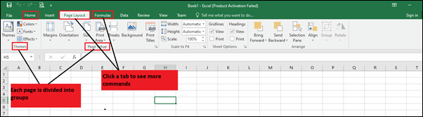
Each tab of Excel Ribbon contains its related operations list. For example, the formula tab contains all the mathematical, logical, text, string, finance, Date, and time functions.

To minimize and maximize the Ribbon

The Ribbon is designed to respond to our current function, but we can choose to minimize it if we find that it takes up too much screen space.

1. To click the Ribbon Display Options arrow in the upper-right corner of the Ribbon.
   
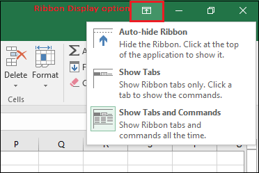
2. Select the desired minimizing options from the drop-down menu:
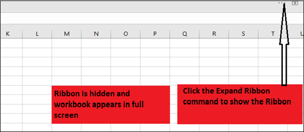
   • Auto-hide Ribbon: Auto-hide shows our workbook in full-screen mode and hides the Ribbon completely. To show the Ribbon, click Expand Ribbon command at the top of the screen.
     
   • Show Tabs: This option hides all command groups when not in use, but tabs will remain there. To show the Ribbon, simply click on any of the tabs.
     
   • Show Tabs and Commands: This option maximizes the Ribbon. All of the tabs and commands will always be visible to the user. This option is selected by default when we open Excel for the first time.
     

To Customize the Ribbon in Excel 2016

We can customize the Ribbon by creating our own tabs with whichever commands we want. Commands are always housed within a group, and we can create as many groups as we want to keep our tab organized. If we want, we can even add commands to any of the default tabs, as long as we create a custom group in the tab.

If we want, we can even add commands to any of the default tabs, as long as we create a custom group in the tab.

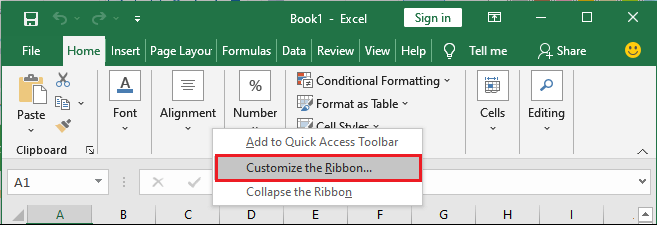
1. Right-click the Ribbon and then choose Customize the Ribbon from the drop-down menu.
   
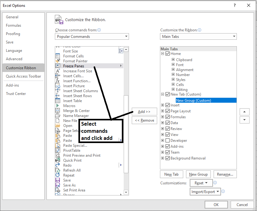
2. The Excel Optionsdialog box will occur. Locate and select New Tab or New group, whichever you want to add.
   
3. Now, select a command from the left panel and click the Add button to the new customized tab/group. You can also drag the commands directly into a group.
   
4. When you are done adding commands, click OK. The commands will be added to the Ribbon in a new tab like this.
   

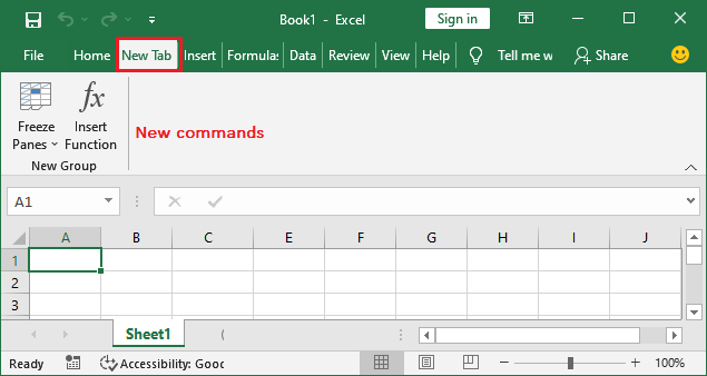
Note: You can also rename the tab and group name.

Formula Bar

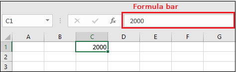
In the formula bar, we can enter or edit data, a formula, or a function that will occur in a specific cell. It allows to write the function and formulas to manipulate the data.

In the image below, cell C1 is selected, and 2000 is entered into the formula bar. Note how the data contains in both the formula bar and in cell C1.

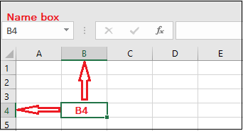
Name Box

The Name box presents the location or "name" of a selected cell.

In the image below, cell B4 is selected. Noted that cell B4 is where column B and row 4 intersect.

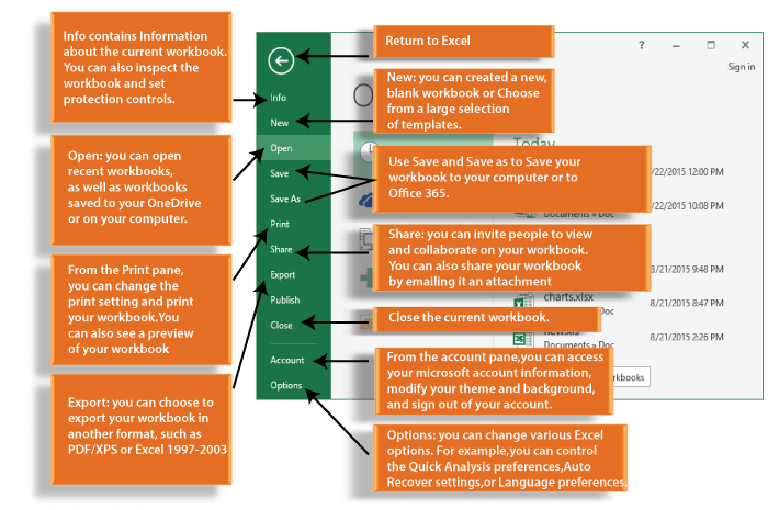
The Backstage View (The File Menu)

Click the File tab on the Ribbon. The Backstage view will emerge.

It is the backstage view of MS Excel and information about the options it contains.

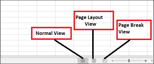
The Worksheet Views

Excel 2016 has a variety of displaying options that change how our workbook is showed. We can choose to view any workbook in the Normal view, Page Layout view, or Page Break view. These views can be useful for several tasks, especially if we're planning to print the spreadsheet.

To change the worksheet views, locate and choose the desired worksheet view command in the bottom-right corner of the Excel window.

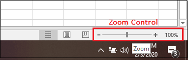
Zoom Control

To use a Zoom control, click and drag the slider. The number to the right of the slider reverse the zoom percentage. It presents at the bottom right corner of the Excel worksheet.

 

                                                                BASIC FORMULAS

Excel formula

Excel formula refers to the formulas used for various calculations. Let's first discuss the concept of formula.

What is the formula?

A formula is a set of mathematical elements that specify a rule. It connects one or more elements with an equal sign. The formula can be used to find the element's value if one or more elements are known.

For example,

Sum = a + b

If we know the value of a and sum, we can find the value of b (b = Sum - a). Similarly, if we know the value of a and b, we can find the sum (sum = a + b).

Or

Mean = Sum of all the observations/ Number of observations

The above formulas consist of three elements. If we know the value of any two elements, we can easily find the value of third element.

What is a formula in excel?

The formula in excel is calculated based on the cells enclosed within the brackets of the function. It means that these formulas have two parameters, function name and the cells declared in a function. For example, B + C + D find the sum of the range of values from B to D. The format of the functions defined in excel as a formula is given by:

Function (cell range1: cell range2)

Where,

Function: It defines the predefined formula in excel, such as SUM and AVERAGE. The names given to the function are familiar.

For example,

SUM (B1: B4)

Here, B1 and B4 are the cell range. The SUM() function will sum all the values from B1 to B4. Similarly, other formulas in excel are defined based on the same concept.

Automatic search for formulas

Excel also provides us an option to find the available functions formulas in the form of a list. So, if anyone is not aware of the available formulas, it is best to find the available formulas in excel quickly. It is given by:

'Insert function'

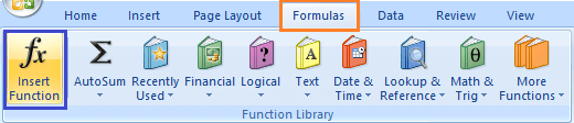
We can find this function under the formula option present on the tool bar. To operate, consider the below steps.

1. On the excel home page, click on the Formulas option present above the toolbar -> click on the Insert function option, as shown below:
   
2. A dialogue box will appear.
3. We can select the functions from the list, as shown above.
   We can also search for a function by specifying the statement for the corresponding function. For example,
   We need to find the minimum value, but there is no function present in the function list. So, we can specify the statement 'to find the minimum value' and press on the 'Go' option. The functions according to the specified statement will appear in the function table, as shown below:
   
   We can use the appropriate function from the table to find the minimum value.
   Similarly, other functions can be easily found by specifying the related statement.

Note: Excel provides a detailed explanation of the given formula. It can be seen on the bottom of the function dialogue box. The statement related to the formula will also appear when we type a function on the formula bar with an equal (=) sign mentioned at the beginning.

Formulas in Excel

Let's discuss the most common formulas in excel. We will also discuss examples based on each formula.

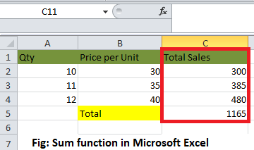
1. SUM ()

The sum function is used as the addition function. It is used to add two or more than two numbers. The addition using excel is quick as compared to the calculator. We can add hundreds or thousands or more numbers easily using the sum function.

Shortcut Method

The AutoSum symbol available on the toolbar can be directly used to add the selected numbers in a single click. It is present on the toolbar under the formula tab.

Example 1: To find the sum of Price of various products.

Consider the below steps to find the sum.

1. Click on any cell outside the given table.
2. Drag the mouse on the formula bar and type '=SUM(C5:C11).' Here, C5 and C11 are the name of the first and last element of the price column. Excel will add the numbers from C5 to C11.
3. Press Enter. The sum will appear on the specified cell, as shown below:
   

OR

1. On the excel home page, select the numbers to be added with the help of a cursor.
2. Click on the AutoSum option under the formula tab, as shown below:
   
3. The sum will appear beneath the cell of the last element.

Example 2: To find the sum of specific elements of the column.

Consider the below steps:

1. Click on any cell outside the given table.
2. Drag the mouse on the formula bar and type '=SUM(C5:C7,C9,C11).' Here, the sum will be calculated of cells C5, C6, C7, C9, and C11. The selected cells for addition are shown below:
   
3. Press Enter. The sum will appear on the specified cell, as shown below:
   

Note: We can type the formula either on the formula bar or on the specified cell. The formula will appear at both the places (formula bar and the specified cell).

2. Subtraction

It is similar to the addition process. We only need to insert a negative sign behind the number we want to subtract.

The formula is given by:

SUM(cell1, -cell2)

For example,

SUM(A1, -A3)

The above formula will be used to subtract value of cell A3 from A1. It will be considered as A1 - A3.

Let's consider an example.

Example: To find the difference between the change in prices of commodities.

Consider the below steps:

1. Click on the first cell of the difference column, as shown below:
   
2. Drag the mouse on the formula bar and type '=SUM(D3, -C3).' The value of cell C3 will be subtracted from the value given in cell D3.
3. Press Enter. The difference between two specified cells will appear. It is shown below:
   
   Similarly, we can find perform the subtraction of multiple cells.

3. Multiplication and Division

A particular name does not specify these formulas. We can directly use the multiplication and division symbol between the two numbers to compute multiplication and division.

It is given by:

A1 * A2

A1 / A2

Let, A1 = 4, and A2 = 2.

Multiplication = A1*A2 = 4*2 = 8

Division = A1/A2 = 4/2 = 2

Let's understand it with an example.

Example: to find the multiplication of two values in columns A and B.

Consider the below steps:

1. Click on the first cell of the multiplication column.
2. Drag the mouse on the formula bar and type '=C3*D3.'
3. Click on the bottom-right corner of that block and drag to the last cell of the multiplication column.
4. Press Enter. The result will appear on all the specified cells of the column. It is shown below:
   

Now, we will consider the same steps for the division. We only need to insert the formula = 'C3/D3.' It is shown below:

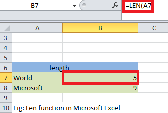
4. LEFT, MID, and RIGHT

These three formulas are used to break down the cell into different segments. Let's discuss this in detail.

LEFT

The LEFT formula is used to extract the starting elements from the specified cell. It is given by:

LEFT(text, Number_of_characters)

Where,

Text refers to the specified cell from which we want to extract the elements.

Number_of_characters refers to the characters we want to extract from the starting from the left most character.

MID

The MID formula is used to extract the number of elements in the middle position from the specified cell. It is given by:

MID(text, start position, Number_of_characters)

Where,

Text refers to the specified cell from which we want to extract the elements.

Start position refers to the position from where we want to start extracting.

Number_of_characters refers to the characters we want to extract.

RIGHT

The RIGHT formula is used to extract the number of elements from the last or right-end. It is given by:

RIGHT(text, Number_of_characters)

Where,

Text refers to the specified cell from which we want to extract the elements.

Number_of_characters refers to the characters we want to extract starting from the right-end character.

Let's consider an example for better understanding.

Example:

Consider the below table in excel.

The steps to extract the characters are as follows:

1. Click on the first cell of the First column, as shown below:
   
2. Drag the mouse on the formula bar and type =' =LEFT(B3,4).'
3. Press Enter. The extracted characters from the specified cell will appear.
4. Drag the bottom-right corner of the first cell to the last element. It will now appear as:
   
5. Now, click on the first cell of the Middle column and type formula =' =MID(B3,5,3)' and press Enter.
6. Similarly, click on the first cell of the Last column and type formula = '=RIGHT(B3,1)'and press Enter.
7. Drag the bottom-right corner of the first cell to the last element of both Middle and Last column. The extracted characters will appear as:
   

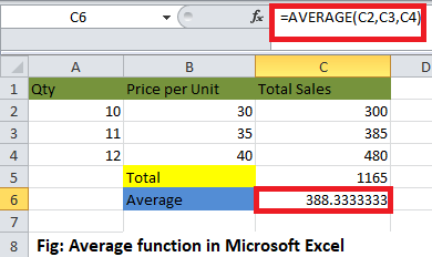
5. AVERAGE

The average function is same as the mean function of mathematics. It is used to find the average of the selected numbers or cells. We can calculate the average of multiple numbers easily.

It is given by:

AVERAGE(number1, number2,....)

In case of range of cells, we can specify it as:

AVERAGE(cell1: cell2)

AVERAGE() is similar to the SUM()/Number of elements in a given column

For example,

AVERAGE(5, 10, 15, 20) = SUM(5, 10, 15, 20)/ 4

Shortcut Method

To access the average symbol, select the numbers with the help of cursor -> click on the drop-down arrow in front of the AutoSum symbol under the formula tab and click on the Average option. The desired average will appear beneath the selected number cells, as shown below:

We can also access more functions by clicking on the 'more functions' option at the bottom.

Example 1: To find the average of the price of the given data table.

Consider the below steps:

1. Click on any cell outside the given table.
2. Drag the mouse on the formula bar and type '=AVERAGE(C5:C9).' Here, the average will be calculated from the range C5 to C9 or (C5, C6, C7, C8, C9).
3. Press Enter. The average of the specified data will appear on the selected cell. It is shown below:
   

The above example finds he average of the elements presents in a particular column. Let's find the average of the elements of a particular row.

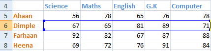
Example 2: To find the average of a particular student of a class.

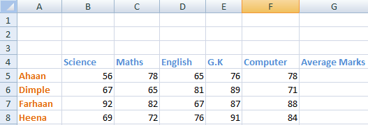
Here, we will find the average marks of the second student Dimple.

Consider the below steps:

1. Click on the second cell under the Average marks column to find the average of a student Dimple.
2. Drag the mouse on the formula bar and type '=AVERAGE(B6:F6).' Here, the average will be calculated from the range B6 to F6 or (B6, C6, D6, E6, F6). The specified range is shown below:
   
3. Press Enter. The average of the specified data will appear on the selected cell. It is shown below:
   
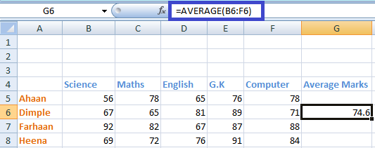
   We can calculate the percentage of rest of the students by dragging downside the bottom-right corner of the cell.

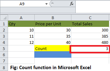
6. COUNT

Count function is used to count the number of data cells in the specified column or row.

COUNT(number1, number2,....)

In case of range of cells, we can specify it as:

COUNT(cell1: cell2)

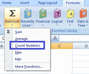
Shortcut Method

To access the count symbol, select the numbers to count-> click on the drop-down arrow in front of the AutoSum symbol under the formula tab -> click on the count option. The desired count will appear beneath the selected number cells. It is shown below:

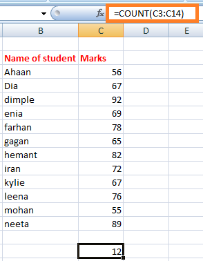
Example 1: To find the count of the number of students in the given data.

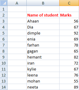
Consider the below steps:

1. Select any cell near the given data table.
2. Drag the mouse on the formula bar and type '=COUNT(C3:C14).' Excel will count the cells from C3 to C14.
3. Press Enter. The counts will appear on the selected cell. It is shown below:

Similarly, we can count the number of elements in a row or column.

Note: he SUM(), AVERAGE(), and COUNT() can only be applied to the list of numbers. It cannot be applied to the data in the form of alphabets. If applied, it will not consider that data or will return 0 as a result.

But, what to do if we want to count the cells with alphabets, such as names of students, name of objects, etc. To resolve this, we have a function named COUNTA(). It can count numbers, alphabets, etc. It means that it can count the cells irrespective of the data inside it. It will also ignore the empty spaces in between.

COUNTA

COUNTA() function is similar as COUNT(). Unlike COUNT(), it can count the cells containing data other than the numbers. Let's consider an example.

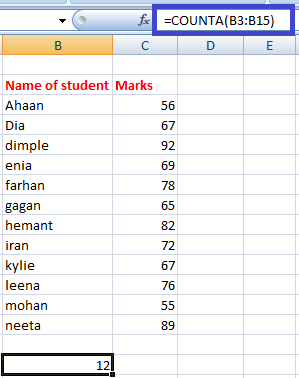
Example 2: To count the number of students with respect to their names.

In the above example, we have counted in terms of the marks of students. But, here we will count with respect to the names.

Consider the below steps:

1. Select any cell near the given data table.
2. Drag the mouse on the formula bar and type '=COUNTA(B3:B15).' Excel will count the cells from B3 to B15. The B15 cell is empty. Thus, excel will ignore the extra space and will count the rest of the cells.
3. Press Enter. The counts will appear on the selected cell. It is shown below:
   

7. MAX and MIN

The MAX() function find the maximum value, and the MIN() function finds the minimum value from the specified data of an array or table.

MAX(number1, number2,....)

In the case of the range of cells, we can specify it as:

MAX(cell1: cell2)

In the case to find the minimum value, the formula is given by:

MIN(number1, number2,....)

In the case of the range of cells, we can specify it as:

MIN(cell1: cell2)

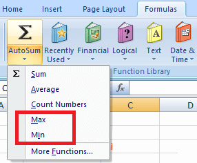
Shortcut Method

To access the MAX()/MIN() symbol, select the numbers-> click on the drop-down arrow in front of the AutoSum symbol under the formula tab -> click on the Max()/Min() option. The desired maximum or minimum number from the selected numbers will appear. It is shown below:

Example 1: To find the topper of the class.

The topper of the class would score highest marks among all the students. Thus, we need to find the average marks from the list of available students.

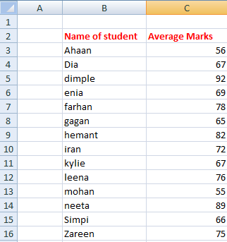
Consider the below steps:

1. Select any cell near the given data table.
2. Drag the mouse on the formula bar and type '=MAX(C3:C16).' Excel will find the maximum value from the range of values between C3 to C16.
3. Press Enter. The maximum value will appear on the selected cell. It is shown below:

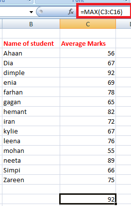
Thus, the student named Dimple is the topper of the class with the highest marks of 92.

Example 2: Find the student with least marks.

Here, we need to find the minimum average numbers of a student from the list of students. The data is the same as in example 1.

Consider the below steps:

1. Select any cell near the given data table.
2. Drag the mouse on the formula bar and type '=MIN(C3:C16).' Excel will find the minimum value from the range of values between C3 to C16.
3. Press Enter. The minimum value will appear on the selected cell. It is shown below:

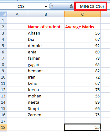
Thus, the student named Mohan scored the least marks (55) in the class.

8. TRIM

The TRIM() function removes the empty spaces between the data in the given array. It is quite useful when we want to arrange the large data in a sequential order without any extra spaces. But, the TRIM() formula can only be applied to a single cell at a time. We can further calculate by dragging down the bottom-right corner of that cell.

The formula is given by:

=TRIM(cell)

For example, TRIM (A2)

Let's consider an example.

Example: To remove the extra space from the given data.

Here, we will use the TRIM() formula to remove the extra spaces.

Consider the below steps:

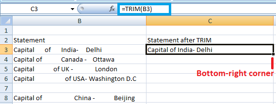
1. Click on the first cell of the second column (C).
2. Drag the mouse on the formula bar and type '=TRIM(B3).' The TRIM() formula here will remove all the extra spaces between the words in the specified cell.
3. Press Enter. The specified statement after the removal of extra spaces will appear on the specified cell, as shown below:
   
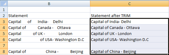
4. Drag the bottom-right corner of that cell to the last cell of the column C. The TRIM() formula will be applied automatically to the other cells beneath it, as shown below:
   

9. IF

The IF() function is used to sort the given data s per the logic. It means that excel check the logic specified within the IF() function.

The formula is given by:

IF(logic, [value_if_true], [value_if_false])

The above formula specifies that if the logic specified is correct, excel will return the value specified in [value_if_true]. If the logic specified is incorrect, it will return

[value_if_false].

For example,

Let, A = 5, and B = 7 and the formula = IF(A >B, True, False)

Output = False

Explanation: The logic specified in the function is incorrect because A is less than B. Hence, excel will return the value False.

If the formula is IF(A >B, 1, 0), it will return 0 because the value specified in the case of false logic is 0.

But, there are some errors to be avoided using the IF() formula, which are listed as follows:

• The declared value in place of true and false, should either be a number or alphabet. We can write it as IF(C2>D3, 1, False), but cannot write is as IF(C2>D3, 1, False0).
• There should be no space between two or more numbers specified in place of true and false. We can write it as IF(C2>D3, 12, False), but cannot write is as IF(C2>D3, 1 2, False).
• We cannot use any other word in place of true and false. We can only use numbers without spacing.

Similarly, we can set the desired value to return in the above formula.

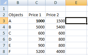
Example: To find if price1 is greater or price 2 with the help of IF() formula.

Consider the below steps:

1. Click on the cell at the end of the first row, as shown below:
   
2. Type the formula '=IF(D3>C3, 1, 0)' on the specified cell.
3. Press Enter. If the statement is true, 1 will appear otherwise 0.
4. Drag the bottom-right corner of the cell to the last element of the table, as shown below:
   
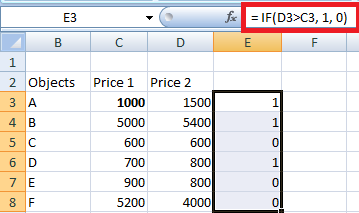
   The corresponding result will appear on other cells as well.

It depicts that the statement with 0 depicts a false statement and 1 depicts a true statement.

Similarly, we can implement multiple formulas using the 'automatic search for formulas' method discussed above.

Note: Remember to insert an equal sign (=) before every formula.

10. PROPER

The PROPER formula is used to organize the names or the words in a standard manner. It means that the first word in a cell must begin with a capital letter. In case the first letter is small; the PROPER formula can be used to organize such words when there is a large volume of text present in excel.

Let's understand with the help of an example.

Consider the below steps:

1. Click on the first cell of the Proper column, as shown below:
   
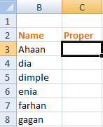
2. Type the formula on the specified cell as' =PROPER(B3).'
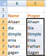
3. Press Enter. The proper form of the given name will appear. It will be the same word, but with the first letter as Uppercase. If the first letter is already in uppercase, no changes will occur. Drag the cursor to the last element of the column, as shown below:
   

11. RANDBETWEEN

The RANDBETWEEN formula generates a random number between the specified numbers. It is given by:

RANDBETWEEN(bottom, top)

For example,

RANDBETWEEN(1,10)

It will display a random number between 1 and 10. It can be any number. It is generally used to find a lucky draw number in excel among various students or names in excel. We only need to type the formula in the form of '=RANDBETWEEN(bottom, top).' We can set any range as per the requirements.

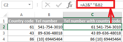
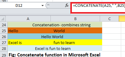
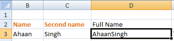
12. CONCATENATE

The CONCATENATE formula can join two or more cells and combine it into one cell. The data to be combined can be in the form of alphabets or numbers. It is given by:

CONCATENATE(cell1, cell2)

Let's consider an example.

The steps are as follows:

1. Click on the first cell of the column concatenate, as shown below:
   
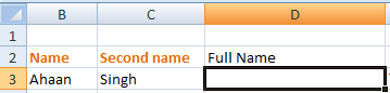
2. Type the formula '=CONCATENATE(B3, C3)' on the cell and press Enter. Here, B3 and C3 are the specified cell numbers.
3. The specified cells in the formula will be combined together, as shown below:
   
   Similarly, we can join multiple cells.

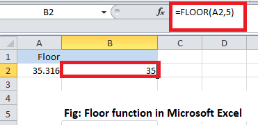
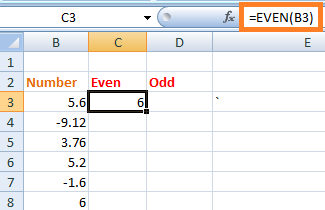
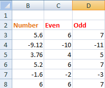
13. EVEN and ODD

The EVEN function rounds off the decimal value to a near even number, and the ODD function rounds off the decimal value to the near-odd number. The same condition applies when we are working with negative numbers. In case of an integer, it will also be converted to the nearest even or odd number.

It is given by:

EVEN (cell_number) and ODD (cell_number)

Here, cell number refers to the value that we want to convert into even or odd.

Let's consider an example.

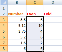
Consider the below steps:

1. Click on the first cell of the even column.
2. Type the formula '=EVEN(B3)' and press Enter. The rounded off value will appear, as shown below:
   
3. Drag down the cursor to the last element of the table. All the specified values in the table will be rounded off to the nearest even number, as shown below:
   
4. Similarly, type the formula '=ODD(B3)' on the first cell of the odd column, and press Enter. Drag down the cursor to the last element. The rounded value will now appear as:
   

14. TODAY

TODAY formula replaces the need to manually type the current date whenever we open the excel sheet. The formula automatically updates the current date on the specified cell.

It is given by:

TODAY()

We need to specify the above formula on the specified cell as '=TODAY()' and simply press Enter.

We are not required to specify anything inside the parenthesis. Every time we open the excel sheet, the date will be automatically updated.

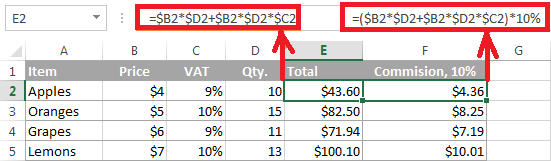
15. Converting Numbers into the currency

The method to specify the same amount in terms of dollars can be accomplished with just a simple click. The shortcut method is given by:

Ctrl +Shift + $

The converted value will be complete in the form of commas, dollar sign, and the decimal point.

Let's understand with the help of an example.

Consider the below steps:

1. Select the given data under the Price1$ column, as shown below:
   
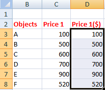
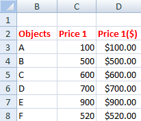
2. Press Ctrl +Shift + $.
3. The select values in the form of numbers will be converted into dollar form, as shown below:
   

Similarly, we can use Ctrl +Shift + % to convert the corresponding values in percentage. In such case, the values will be automatically multiplied by 100 with a percentage symbol.

Complex Formulas

The complex formula refers to the mixed use of addition, subtraction, multiplication, and division formulas. We will simply compute the formula on the formula bar and excel will produce the desired result in few seconds. We can create multiple complex formulas based on the above formulas.

Let's consider an example.

Example: To compute the equation and find out the value.

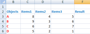
Consider the below steps:

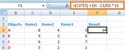
1. Click on the first cell of the result column.
2. Drag the mouse on the formula bar and type '=(C3*E3) + D3 - C3/D3 * E3.'
3. Press Enter. The result will appear on the specified cell, as shown below:
   
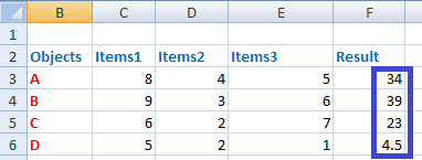
4. Drag the cursor of the first cell to the last cell of the result column. The resulted value will appear on all the specified cells, as shown below: